Long run average and marginal cost curves

1-Explain the derivation of long run average cost curve.

Ans: Long-run average cost is the per unit production cost in the long run. It is calculated by dividing the long-run total average cost by units of output produced in the long-run. Symbolically, long run average cost is expressed as follows.

`LAC= frac{LTC}{Q}`

Where- LAC=Long-run average cost

LTC=Long-run total cost

Q =Units of output

Long-run average cost is derived from the short-run average cost curves. As we know that long-run is the period of time in which the firm can change all of its factors of production and also can change the scale of production. Therefore, in the long-run, the firm does not stick with the existing plant as it does in the short-run. It can install more than a single plant and increase the production of goods and services.

In order to understand the derivation of the long-run average cost curve, let’s consider the short-run average cost curves as shown in the following figure.

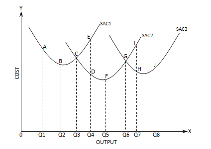
In the figure, output is measured on X-axis and average cost on Y-axis. There are three SAC curves each representing short-run average costs incurred from the use of three different sizes of plants. The firm produces 0Q1 amount of output at AQ1 per unit cost by using the existing plant. When there is an increase in demand for goods, the firm increases in its production from 0Q1 to 0Q2 and 0Q3 in the short time period by increasing variable factors of production. If demand for goods further increases, it decides to increase in production from 0Q3 to 0Q4 amount of output. However, the existing plant incurs higher per unit production cost equal to EQ4 in comparison with per unit cost equal to DQ4. The per unit cost DQ4 occurs only from the use of a second plant. Obviously the firm can minimize the per unit production cost by using the second plant. Therefore, the firm installs new plants in the long run to increase its output at a lower per unit production cost. When the firm produces 0Q5 units of output, the new plant incurs the per unit cost (SAC) equal to FQ5. Further, with the increase in production, the SAC increases and the firm decides to install another new plant or say third plant. While producing 0Q7 amount of output, the third plant is more preferable than the second one because it incurs per unit production cost only equal to HQ7.

This is how the firm does not stick to the existing plant in the long run. It installs bigger and more advanced plants to minimize per unit production cost when it needs to increase its output. By comparing per unit production cost (SAC) of each of the plants, the firm decides to operate to produce required levels of output at minimum possible cost.

In this way, there are different SAC curves of different sizes of plants in the long run. By drawing a smooth line covering the SAC curves in such a way that the line is tangent to the lower portion of each of the SAC curves, we derive the LAC curve as shown in the above figure. In fact, LAC envelopes all SAC curves and sometimes it is called envelope curve as well.

2- Why is long run average cost curve 'U' shaped?  Explain.

Or

Explain the economies and diseconomies of scale of production.

Ans: The long run average cost curve (LAC) first falls slowly and then rises gradually after a minimum point is reached. Initially, it falls because of economies of scale and after it reaches its minimum level it gradually rises due to diseconomies of scale. So economies and diseconomies of scale are mainly responsible for the U-shaped LAC curve as shown in the figure.

In the figure, the LAC curve slowly slopes downward until it reaches point A and thereafter it gradually slopes upward with the increase in the amount of output. This way it becomes U-shaped because of economies and diseconomies of scale.

The economies and diseconomies of scale, which are responsible for the U-shaped LAC curve, are explained in detail below.

1- Economies of Scale

Economies of scale refer to the fall in LAC due to increase in the size of plants in the long run. Economies of scale are of two types as internal & external economies.

1.1- Internal Economies

Internal economies refer to the fall in LAC as a result of the internal performance of the firm in production, distribution, management etc. Internal economies can be explained under the following heads.

a-Economies in Production

Economies in production arise from technological advantages and advantages of division of labor.

When the scale of production is expanded, the firm can have the opportunity to avail advantages of advanced technology. The advanced technology can have the whole process of production of a good in one composite unit of production that helps to minimize per unit cost. For example, a fine flour mill can adopt the technology which peels off wheat grains, grinds, filters and packs fine flour in sacks itself in one composite unit of production. All these processes in one composite unit of production minimizes per unit production cost and the LAC curve slopes downward.

With the expansion of scale of production, more workers of varying skills are employed and they are entrusted with the piece of work to perform where they are best suited. This is known as division of labor. Division of labor leads to specialization and increases productivity. Consequently LAC falls.

b-Economies in Marketing

With the increase in scale of production, the firm can enjoy economies in marketing. Normally, the large-size firms make bulk purchases of raw materials and other inputs. As firms purchase large quantities of inputs, they can get discounts. Consequently, LAC falls resulting in a LAC curve slope downward.

Similarly, firms can enjoy economies in marketing their own products while distributing large quantities at low per unit cost, low advertising cost for increasing quantity of goods etc. all these make LAC fall.

c-Managerial Economies

Managerial economies, with increase in scale of production, arise when the management is divided into specialized departments under specialized personnel and each department is decentralized for decision making. This increases the efficiency in management and enables the department heads to make quick and appropriate decisions in time. Consequently costs resulting in a delay in decision making can be minimized.

d-Economies in Transport and Storage

Large scale firms can also enjoy economies in transport and storage. It is because the large scale firms keep their own means of transport which can be utilized at any time for carrying in raw materials and for carrying out finished goods at a cheaper rate compared to market rate of transport.

Likewise, large scale firms can build their own godowns in the various centers of product distribution and can save on cost of storage.

1.2- External Economies

External economies refer to fall in LAC as a result of the advantages arising outside the firm. Firms with large scale of production, can have economies in the form of discounts and concessions on purchase of inputs, loan facilities from commercial banks at lower rate of interest, establishment of ancillary industries nearby which supply inputs, large scale of hiring means of transport and godowns etc. All these facilities are available for the firms when they operate on a large scale and can reduce per unit cost of production.

2- Diseconomies of Scale

Diseconomies of scale refer to the rising in LAC as a result of increase in size of plant and level of output. Diseconomies of scale are also of two types as internal & external diseconomies.

2.1- Internal Diseconomies

Internal diseconomies refer to the rise in LAC as a result of inefficiency in management, labor inefficiency etc. with increase in size of firms. The responsible factors causing internal diseconomies are explained under the following headings.

a-Managerial Inefficiency

Managerial inefficiency appears with the increase in scale of production to the large extent. There is a vast management which lacks personal contact and communication between owners and managers as well as managers and laborers. In this situation, decision making and implementation of decisions are delayed due to coordination problems. It creates managerial inefficiency which leads to increase in production cost. As a result LAC increases resulting in a LAC curve slope upward.

b-Labor Inefficiency

With the increase in scale of production to a large extent, demerits of division of labor appear due to the feeling of monotony of doing the same type of work for a long period of time, loss of responsibility, lack of joy, disputes among laborers etc. On the other hand, labor unions pressurize management to ensure more facilities for workers. This causes conflicts between workers and management. Such a situation in firms creates an environment of tension which causes a loss of output in per unit of time and hence increase in production cost. As a result LAC increases leading to LAC curve slope upward.

2.2- External Diseconomies

External diseconomies refer to the increase in LAC of production as a result of disadvantages that appear outside the firm with the increase in scale of production. When all firms of the industry are expanding, the discounts and concessions available on bulk purchase of inputs come to an end and input-prices increase because of the competition of rival firms for purchasing the same variety of inputs. On the other hand, easy loan facilities by commercial banks are also put to an end. The law of diminishing returns to scale comes into force due to excessive use of fixed factors. Due to natural constraints, the extractive industries also get exhausted. All these reasons are responsible for the increase in production cost in the long run.

3- Is the long run average cost curve always ‘U’ shaped?

Ans: No, the long run average cost curve is not always U-shaped. Traditionally, it was believed that the LAC curve is U-shaped but many empirical studies have proved that the LAC curve is L-shaped. The empirical studies show that diseconomies of scale which cause an increase in production cost in the long run can be avoided by technological progress in production. Technological progress along with sustainable production practices enables the firms to maintain the cost of production at a minimum level in the long run. Initially, economies of scale make the LAC curve first to slope downward and when it reaches its minimum level then remain flat, that makes the LAC curve L-shaped.

4- Explain the derivation of long run marginal cost curve.

Ans: The long-run marginal cost is equal to the change in long-run total cost as a result of change in output in the long run and is expressed as,

 `LMC=\frac{ΔLTC}{ΔQ}`

Where, `LMC`  =Long run marginal cost,

`ΔLTC`=Change in long run total cost,

`ΔQ`     =Change in output produced,

Long run marginal cost curve (LMC) is derived from the short run marginal cost curve (SMC). In order to understand the derivation of the long run marginal cost curve, let’s consider the following figure.

In the figure, first let’s consider the points of tangency of the long run average cost curve to each of the short run average cost curves denoted by A, B & C. The LMC equals to SMC for the output at which the LAC curve is tangent to the corresponding SAC curve. Now draw perpendiculars to X-axis from the points of tangency A, B & C to find SMC for each of the amounts of output 0Q1, 0Q2 & 0Q3. The perpendicular drawn from point A intersects SMC1 at point L, hence SMC for 0Q1 amount of output is equal to LQ1 which is also equal to LMC for the same amount of output. When the amount of output is increased to 0Q2, the perpendicular drawn from point B shows SMC is equal to BQ2 which is also equal to LMC for 0Q2 amount of output. Likewise, if the output is further increased to 0Q3, the perpendicular drawn from point C is extended up to point N where SMC for 0Q3 amount of output is equal to NQ3. This NQ3 is also equal to LMC for the same amount of output. If all these points L, B & N of SMC for different amounts of output are joined together with a line, we drive the LMC curve for different amounts of output as shown by the blue dotted line in the figure.